The Singular Value Decomposition

Lecture notes · about 15 min · last revised 2026-05-02

1 From eigenvectors to singular vectors

Eigenvectors are the natural coordinates of a square matrix, but they have two practical defects: not every matrix is diagonalizable, and eigenvectors of a non-normal matrix need not be orthogonal. The singular value decomposition sidesteps both problems by describing how a matrix acts on pairs of orthonormal bases — one for the input space and one for the output space.

The price is small: instead of an equality Av = λv we ask for the weaker, and always attainable, relation

A v i = σ i u i, σ 1 \geq σ 2 \geq \dots \geq σ r > 0,

where {u_i} and {v_i} are orthonormal sets. The scalars σ_i are the singular values, the v_i are right singular vectors, and the u_i are left singular vectors.

2 Definition and existence

Definition (SVD)

Let A ∈ ℝ^m×n with rank r. A singular value decomposition of A is a factorization

A = U Σ V T

where U ∈ ℝ^m×m and V ∈ ℝ^n×n are orthogonal, and the diagonal of Σ ∈ ℝ^m×n contains σ₁ ≥ … ≥ σ_r > 0 = σ_r+1 = ….

Existence follows from the eigendecomposition of the symmetric positive semidefinite matrices A^TA and AA^T: both share the eigenvalues σ_i², and pairing their eigenvectors yields the relation above. Alternatively, a compact variational argument defines each singular value by a max–min principle, σ_k = max_{dim S = k} min_{0 ≠ x ∈ S} ‖Ax‖ / ‖x‖, which makes no reference to eigenvectors at all.

Two identities follow immediately and are worth memorizing: the spectral norm is the largest singular value, ‖A‖₂ = σ₁, and the Frobenius norm collects them all, ‖A‖_F² = ∑_i σ_i².

3 The geometry

Read right to left, A = UΣV^T says that every linear map is the composition of a rotation, an axis-aligned stretch, and a second rotation. The unit sphere is mapped to an ellipsoid whose semi-axis lengths are exactly the singular values.

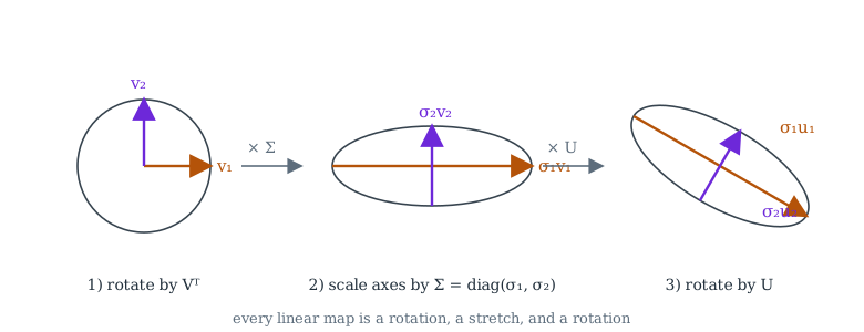
Figure 1. The three geometric stages of the SVD of a 2×2 matrix. Singular values are the semi-axes of the ellipse.

Remark

The figure also explains the determinant: rotations preserve oriented area, so |det A| = σ₁σ₂ — the area of the image of the unit square.

4 Best low-rank approximation

Truncating the decomposition after k terms produces

A k = \sum i=1 k σ i u i v i T,

a rank-k matrix. The celebrated theorem of Eckart and Young says this truncation is optimal in every unitarily invariant norm.

Theorem (Eckart–Young–Mirsky)

For every matrix B of rank at most k,

‖A - A k ‖ 2 = σ k+1 = min rank B \leq k ‖A - B‖ 2 .

The same holds for the Frobenius norm, where the error is √(σ_k+1² + …).

The practical consequence is a compression law: if the singular values decay quickly, then A is — to within noise — a low-rank object, and storing k(m+n) numbers instead of mn loses almost nothing. Which matrices have fast decay, and how to find the dominant subspace without ever forming A^TA, is the subject of the research notes on randomized approximation.

5 Computing the SVD

Dense solvers (LAPACK's gesdd) reduce the matrix to bidiagonal form by orthogonal similarity transformations — Golub–Kahan's two-sided Householder scheme — and then resolve the bidiagonal problem by a variant of the QR algorithm or by divide-and-conquer. Complexity is O(mn·min(m,n)), which is fine for a matrix that fits in memory but prohibitive when A is an operator known only through matrix–vector products. In that regime one turns to iterative methods: Lanczos bidiagonalization for the extreme singular values, or randomized range finders for the dominant subspace.

6 Applications

Conditioning. The ratio κ(A) = σ₁/σ_n bounds the amplification of errors when solving linear systems; it is the right way to say a matrix is "almost singular".
Principal component analysis. PCA of centered data is the SVD of the data matrix; the scores, loadings, and explained variance all come from one decomposition.
Compression and denoising. Truncated SVD underlies image compression, latent semantic indexing, and optimal hard-thresholding denoising.
Pseudoinverse and least squares. The Moore–Penrose pseudoinverse is A⁺ = VΣ⁺U^T, and cutting small singular values regularizes ill-posed least-squares problems.
Rank detection. Numerical rank is the number of singular values above a tolerance scaled by σ₁ and machine precision.

References

G. H. Golub, C. F. Van Loan, Matrix Computations, 4th ed., Johns Hopkins University Press, 2013, Chapter 2 and §8.6.
L. N. Trefethen, D. Bau III, Numerical Linear Algebra, SIAM, 1997, Lectures 4–5 and 35.
C. Eckart, G. Young, "The approximation of one matrix by another of lower rank," Psychometrika 1 (1936), 211–218.
N. Halko, P.-G. Martinsson, J. A. Tropp, "Finding structure with randomness," SIAM Review 53 (2011), 217–288.