Eigenvalues and Spectral Theory
1 Eigenvalues and eigenvectors
Geometrically, an eigenvector is a direction the matrix leaves invariant — it may stretch or flip the line, but not turn it. A generic vector has no such privilege, as the figure shows.
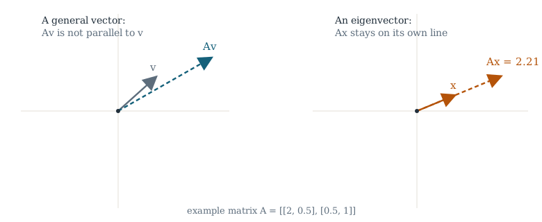
Figure 1. For A symmetric, most vectors change direction under A; eigenvectors (right) keep their line and are simply rescaled.
2 The characteristic polynomial
The eigenvalues are the roots of p(λ) = det(A − λI), a degree-n polynomial. Over ℂ the matrix is always triangularizable; over ℝ complex pairs appear whenever p has non-real roots. Although the characteristic polynomial settles existence, it is a poor numerical route to eigenvalues: root-finding of a degree-n polynomial whose coefficients vary enormously in scale is far less stable than the orthogonal iterations used in practice (QR algorithm, Lanczos). The trace and determinant record the two leading coefficients, giving the familiar identities tr A = ∑ λi and det A = ∏ λi.
3 Gershgorin circles
Before computing anything, it often helps to localize the spectrum. Gershgorin's theorem gives a cheap inclusion region using only the entries of the matrix.
A diagonally dominant matrix therefore has all its disks — and hence its whole spectrum — bounded away from zero, which already implies nonsingularity.
4 The spectral theorem
For symmetric matrices the theory collapses to something almost perfect.
Every concept in these notes specializes cleanly in the symmetric case: singular values are the absolute values of eigenvalues, the numerical range is the interval [λmin, λmax], and iterative methods converge at rates governed by eigenvalue ratios. This is why symmetric problems — discrete Laplacians, Hessian matrices, covariance matrices, graph Laplacians — are the pleasant hemisphere of numerical linear algebra.
5 Perturbation: Weyl's bound
How much can the spectrum move when the matrix is perturbed? For symmetric matrices the answer is reassuringly little.
For nonsymmetric matrices no comparable bound exists: eigenvalues can be hyper-sensitive, since they depend on the entries like the roots of a high-degree polynomial. The picture below contrasts the tame spectra one meets in symmetric problems with the disk-filling spectra of perturbed nonsymmetric ones.
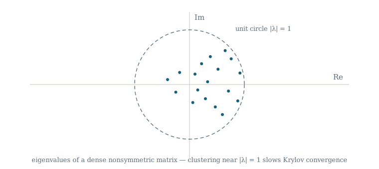
Figure 2. Eigenvalues of a dense nonsymmetric matrix cluster near the unit circle; spectra hugging |λ| = 1 are the classical obstacle to fast Krylov convergence.
6 The power iteration
The simplest eigenvalue algorithm multiplies a random start vector by A repeatedly. Components along eigenvectors with smaller |λ| decay relative to the dominant one at rate |λ2/λ1| per step, so the iterate aligns with v1 and the Rayleigh quotient converges to λ1. Shift-invert accelerates the ratio; deflation and orthogonalization against found vectors extend the method to further eigenvalues — and iterating all vectors simultaneously against their span is precisely what Lanczos and Arnoldi do, which is where the next note begins. You can watch the raw power method converge — and see how the error collapses once the residual direction is clean — in the interactive demos.
References
- R. A. Horn, C. R. Johnson, Matrix Analysis, 2nd ed., Cambridge University Press, 2013.
- L. N. Trefethen, D. Bau III, Numerical Linear Algebra, SIAM, 1997, Lectures 24–27.
- G. H. Golub, C. F. Van Loan, Matrix Computations, 4th ed., 2013, §7.3 and §8.1.
- H. Weyl, "Das asymptotische Verteilungsgesetz der Eigenwerte linearer partieller Differentialgleichungen," Math. Ann. 71 (1912), 441–479.